Playing with Randomness and Interactions to Prove Theorems

This post will explore some (of the many) remarkable results in theoretical computer science and in the field of probabilistic proof systems in particular. While many essential results won’t unfortunately be mentioned, and most details omitted, I will rather focus on providing intuition for concepts and invite the interested reader to explore and study the various resources linked throughout this article for precise definitions and proofs.

Basic knowledge of complexity theory (P, NP classes) (see e.g. this book or this book for great resources on the matter), as well as basic concepts of abstract algebra (groups, rings, fields).

Informally a proof system $\mathcal{S}$ is the composition of an axiomatic system (a finite set of statements taken to be true – called axioms) along with a set of inference rules. These rules determine the set of transformations that can be carried out on the information within the system, with axioms as a staring point (see here for more details).

On input a set of premises, an inference rule outputs a consequence that is then added to the set of information (“expressions”) in the system.
We call a proof $\pi$ for a theorem $\mathcal{T}$ in the proof system $\mathcal{S}$, a sequence of expressions such that:

• the first expression is an axiom,
• the last expression is the theorem $\mathcal{T}$, and
• all intermediate expressions are either axioms or expressions obtained by sequential application of inferences rules from an axiom.

Intuitively, a proof system may be modeled as a set of initial states (the axioms), and a set of state transitions (the inference rules), in which all provable theorems are the final states of the set of all finite-state automaton obtained by sequentially applying state transitions from the initial states. The proof of a theorem can be represented as the sequence of state transitions from the initial state (axiom) to the final state (theorem).

While all the above may sound trivial to most readers, several observations are worth highlighting:

• Proofs are hard to find. On a given set of axioms and inference rules, finding a suitable sequence of expressions leading to the theorem is a non-trivial task. For most of us (at least for me!) rigorously proving mathematical theorems requires a lot of work.
• Proofs are interesting. A proof contains a lot of information about the theorem itself. In fact, the proof not only shows that the theorem is true, but it also shows why, which is a very valuable thing to know.
• Proofs are “static”. When a theorem is proven, it is proven. The proof can be written on paper, peer-reviewed and shared. Proofs (in the mathematical sense) are inherently “static”.
• Verifying a proof is “easy”. To verify a proof it is necessary to check that all expressions in the sequence are compliant with the inference rules of the proof system. Hence, verifying a proof is at least as long as reading the proof, which can be long if the proof is long, but remains orders of magnitude simpler than finding the proof in the first place.

In the following, we denote by $\mathbf{R} \subset \{0,1\}^* \times \{0,1\}^*$ a polynomial-time decidable binary relation, and denote by $\mathbf{L} = \{x\ |\ \exists w\ \text{s.t.}\ \mathbf{R}(x, w)\}$ the language defined by the relation $\mathbf{R}$. Further we will refer to $x$ as the “instance” (or “public input”) and to $w$ as the “witness” (or “private input”). (Looking back to the section above, the language $\mathbf{L}$ can be seen as the set of provable theorems in a proof system, while $w$ is their associated proofs. We see that this definition is natural, since, informally, for $x$ to be in $\mathbf{L}$ – i.e. for $x$ to be a provable/valid theorem – there need to exist a proof for it!)

Finally, we use the symbol $\leftarrow$ to represent assignment (e.g. $y \leftarrow 2$ assigns the value $2$ to the variable $y$), while $y \stackrel{\$}{\leftarrow} S$ denotes the action to assign to $y$ a value taken uniformly at random from the set $S$. With this minimal set of notations we are now ready to enter the realm of probabilistic proof systems.

In their seminal work Goldwasser, Micali and Rackoff (GMR) introduced the notion of Interactive Proof Systems, in which a prover $\mathsf{P}$ and a verifier $\mathsf{V}$ – both modeled as Interactive probabilistic Turing Machines – communicate by means of their input and output tapes and exchange a sequence of messages. In the protocol, $\mathsf{P}$ wants to prove to $\mathsf{V}$ that $x \in \mathbf{L}$ (i.e. that a theorem is true). $\mathsf{V}$, on the other hand, wants to make sure that $x$ is a valid instance and so, wants to check that $\exists w\ \text{s.t.}\ \mathbf{R}(x,w)$ (i.e. there exists a correct proof for the theorem). To that end, the verifier is allowed to flip coins (i.e. has access to a source of truly random bits), and uses these coin flips to ask questions (i.e. “send challenges”) to the prover. The prover answers the verifier’s questions, and after several interactions, the verifier decides to either accept or reject the prover’s statement. Importantly, proofs are not “static” anymore in this model, but are now “built on the fly” by the prover via his interactions with the verifier. Informally, the complexity class admitting interactive proofs (IP) is defined as the class of languages $\mathbf{L}$ with the following properties:

• Completeness: “Valid instances are accepted most of time”
  \begin{equation}
  \mathrm{Pr}\left[ \mathsf{V}\ \text{accepts}\ (\pi, x)\ |\ x \in \mathbf{L},\ \pi \leftarrow \mathsf{Transcript}(\mathsf{P}, \mathsf{V}) \right] \geq \frac{2}{3}
  \end{equation}
• Soundness: “Invalid instances are rarely accepted”
  \begin{equation}
  \mathrm{Pr}\left[ \mathsf{V}\ \text{accepts}\ (\pi, x)\ |\ x \not\in \mathbf{L},\ \pi \leftarrow \mathsf{Transcript}(\mathsf{P}, \mathsf{V}) \right] \leq \frac{1}{3}
  \end{equation}

where $\mathsf{Transcript}(\mathsf{P}, \mathsf{V})$ represents the sequences of messages exchanged between the prover and the verifier during the protocol (i.e. the set of verifier’s challenges and the associated answers by the prover). Interestingly, we clearly see that running this probabilistic protocol – for communicating a proof – $N$ times can be used to “amplify soundness”. In short, if after running the protocol $N$ times (sequentially or concurrently) the verifier accepts an invalid instance, this means that during all executions of the protocol the verifier accepted $x$. The probability of this event is $\mathrm{Pr}\left[ A_1\ \land\ \ldots\ \land\ A_N \right]$ (where $A_i$’s are independent and represent acceptance of $x$ by $\mathsf{V}$ in protocol execution $i$). As per the definition of soundness above, this is bounded by $\frac{1}{3^N}$ which converges exponentially fast to $0$ (e.g. if $N = 10$, the probability for $\mathsf{V}$ to be duped already falls to $\frac{1}{59049} \approx 0.000017$!).

Importantly, in the GMR protocol, no assumptions are made on the prover. As such, it is modeled as all powerful/computationally unbounded. The verifier, however, is considered “weak”/computationally bounded.

At this stage, it is legitimate to wonder: How by flipping fair coins and interacting with the prover can the verifier almost always accept valid statements and almost always reject false ones?

The key aspect of this method is that the prover does not know in advance the challenges he will receive from the verifier. As such, it is very hard for him to cheat. More than that, it is actually impossible for the prover to derive any sensible cheating strategy, since the verifier’s challenges are derived from random bits (“the verifier’s coin flips”). As such, and strikingly, communication (i.e. interactions) and randomness seem very powerful.

While interactions allow to convey information and exchange knowledge, randomness is a fundamental tool to build sound protocols at is defeats lying provers’ strategies.

A key method used to design efficient and sound interactive protocols is called: arithmetization.

In short, this method consists in encoding computation so that its correctness can easily be verified via few probabilistic algebraic checks. Informally, such encoding can be done by converting a boolean formula into a polynomial defined over a large prime field and checking the formula’s satisfiability by evaluating the polynomial. A key insight behind the power of this method to represent (and check) computation is that polynomials are great error-correcting codes (e.g. Reed-Solomon codes or Reed-Muller codes. See e.g. here for more information). As such, any error in the initial boolean formula (representing the prover’s computation) “gets propagated all over the resulting polynomial”! What this means is that, when the verifier queries this resulting polynomial, the probability for him to spot a mistake/error in the prover’s computation is very high!

All in all, moving the prover’s computation to the realm of a polynomials defined over large prime fields gives great power to the verifier. Even if modeled as a weak device, the verifier has a lot of chances to discover a “lie in the prover’s statement”. (An illustration of the usefulness of polynomials – especially low-degree extensions – can be found in Justin Thaler’s blog post about the Sum-Check protocol in this series).

Example.

Assume that the prover claims that he knows the first $10$ elements of the Fibonacci sequence. We know that these elements are: $\{0,1,1,2,3,5,8,13,21,34\}$. However, let’s assume that the prover did a mistake when computing the last element and instead has the sequence $\{0,1,1,2,3,5,8,13,21,33\}$. For the sake of this example we assume that we work in the prime field $\mathbb{F}_{101}$, and so, would like to manipulate polynomials in the ring $\mathbb{F}_{101}[x]$.

To get a sense of “the power of polynomials”, we will treat both of these sets as evaluation points of two polynomials. These sets of evaluation points will serve as interpolation domain to recover two polynomials in the coefficient form.

As such, interpolating both

$$\{(0,0), (1,1), (2,1), (3,2), (4,3), (5,5), (6,8), (7,13), (8,21), (9,34)\}$$

$$\{(0,0), (1,1), (2,1), (3,2), (4,3), (5,5), (6,8), (7,13), (8,21), (9,33)\}$$

respectively gives

$$f(x) = 44x^9 + 31x^8 + 43x^7 + 16x^6 + 38x^5 + 52x^4 + 12x^3 + 9x^2 + 59x$$

$$g(x) = 13x^9 + 36x^8 + 85x^7 + 40x^6 + 9x^5 + 4x^4 + 24x^3 + 79x^2 + 14x$$

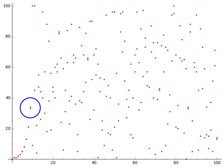
and we know that these two univariate polynomials can coincide on at most $9$ points (see the DeMillo-Lipton–Schwartz–Zippel lemma for more information). Strikingly, a simple representation shift (i.e. interpolation) of seemingly “similar” polynomials reveals a lot of disparities (their coefficient representations are indeed completely different). This in turn, is confirmed when we look at the set of evaluations of these polynomials in the field (see picture), where we see that a simple “tiny error” (blue circle on the figure) made by the prover, ends up being propagated all over the evaluation domain, making it easy for the verifier to check whether the prover’s statement actually holds.

In addition to the interactive method for proving theorems, Goldwasser, Micali and Rackoff also studied the amount of “knowledge” that needed to be communicated between the prover (willing to prove a theorem) and the verifier (willing to accept only valid theorems) in the protocol.

In their work, the authors informally define “communications conveying knowledge” as those that transmit the output of an unfeasible computation, a computation that the verifier cannot perform herself. In fact, does the teacher learn something new when her student gives her a proof of the Pythagorean theorem? She certainly learns that her student is capable to come up with a proof for the theorem; but beyond that, the teacher does not learn anything new (she already was able to come up with a proof for the theorem herself). However, does the teacher learn something if her student sends her a proof of the Riemann hypothesis? Certainly yes! Not only she will learn that the Riemann hypothesis is true, but she will also learn how to prove it! What’s more, if she is malicious, the teacher can try to claim the prize associated to proving this hypothesis.

The, now famous, notion of “zero-knowledge” proof introduced in the same seminal work allows to remedy to the (“malicious teacher”) problem aforementioned. In short, these proofs allow a prover to prove a theorem $\mathcal{T}$ to a verifier without exposing any additional details on “why” the theorem is valid.

Formally, knowledge (resp. zero-knowledge) is captured by using the (theoretical) concept of an extractor (resp. simulator).
These theoretical concepts are embodied by very strong and idealized algorithms. Intuitively, the extractor represents the idea that if you “know” something, I can surely – with some extra powers – extract this knowledge from you. For instance, if I can read your mind, I can surely extract your “knowledge” (alternatively, and less poetically, it is feasible to extract knowledge from a prisoner by using non-conventional and forbidden methods like torture). Either way, if you didn’t “know” something, it would be impossible – not matter how – to extract this thing from you.

The notion of zero-knowledge, however, captures the idea that if a verifier does not learn anything other than the fact that the theorem is true, then he surely cannot distinguish between a legitimate prover, and a simulator which does not know a witness for the instance (i.e. does not know a proof for the theorem), but which is given the possibility to cheat (i.e. a “trapdoor”). If the verifier could distinguish, then he must have learned something beyond the fact that the theorem is valid.
(If that helps, think about a sort of Turing test where a verifier needs to distinguish between a prover having a valid proof and a simulator having a trapdoor that allows him to derive a perfect cheating strategy).

Example: Schnorr protocol.

Let’s illustrate these seemingly mind-boggling notions by looking at a very simple yet extremely powerful example. In fact, let’s build the extractor and simulator for the Schnorr protocol. This protocol is an example of sigma protocol that can be used to prove knowledge of a discrete logarithm.

Let $\mathbb{G}$ be a cyclic group of prime order $q$ with generator $\mathtt{g}$. We denote by $*$ the group operator, and use the “exponentiation” notation to denote its successive application, e.g. $\mathtt{g}^k = \mathtt{g} * \ldots * \mathtt{g}$ ($k$ times). Assuming that $h (= \mathtt{g}^w) \in \mathbb{G}$ and $(\mathbb{G}, q, \mathtt{g})$ are publicly available, the Schnorr protocol allows to prove knowledge of $w$, and goes as follows:

1. The prover computes $a \leftarrow \mathtt{g}^r$, where $r \stackrel{\$}{\leftarrow} \mathbb{Z}_q$; and sends $a$ to the verifier.
2. After reception of $a$, the verifier “flips a coin” and sends a challenge $c \stackrel{\$}{\leftarrow} \mathbb{Z}_q$ to the prover.
3. Upon reception of the challenge, the prover answers with $z \leftarrow c \cdot w + r$.
4. Finally, the verifier accepts (that the prover knows the discrete logarithm of $h$ in base $\mathtt{g}$) if $\mathtt{g}^z$ equals $a * h^c$, and rejects otherwise.

The extractor for this protocol, has the power to control space and time. In fact, to build the extractor, we assume that this algorithm can “rewind” and re-run the prover on the same input while preserving the prover’s random tape. This means that, after rewinding the prover, the same random element $r$ will be selected from $\mathbb{Z}_q$, and so the prover’s first message will be the same. Now, however, the extractor sends a different challenge $c’$ to the prover who will continue its normal execution of the protocol.
This powerful ability to rewind the prover allows to generate two accepting transcripts $(a, c, z)$ and $(a, c’, z’)$ from which it becomes possible to recover the prover’s witness $w$ by observing that $\frac{z-z’}{c-c’} = \frac{(c \cdot w + r) – (c’ \cdot w + r)}{c-c’} = \frac{(c-c’)w}{c-c’} = w$.

To build the simulator for this protocol, we equip this algorithm with the power to see the verifier’s random tape/foresee the verifier’s challenge. As such, with this extra power, it is possible for the simulator to come up with an effective cheating strategy. In fact, knowing the challenge $c$, the simulator’s first message is set to $\mathtt{g}^z * h^{(-c)}$, where $z$ is an arbitrary element of $\mathbb{Z}_q$, also sent in the simulator’s last message. As such, it is clear that the final check $\mathtt{g}^z = \mathtt{g}^z * h^{(-c)} * h^c$ is satisfied (it is a tautology) while the simulator did not know $w$.

Importantly, we note that in order to be able to simulate in this protocol, it is necessary that the verifier is honest, and sends truly random challenges. In fact, since the simulator’s “power” consists in reading the random tape of $\mathsf{V}$, this power is rendered useless if the verifier does not use his tape to create the challenge. This is why we say that the Schnorr protocol is Honest Verifier Zero-Knowledge (HVZK).

We have illustrated in this example the notions of an extractor – used in proofs of knowledge (in which the prover not only shows that $\exists w\ \text{s.t.}\ \mathbf{R}(x,w)$ but that he knows such $w$) – and the notion of a simulator – used to prove the zero-knowledge property.
Surely, these algorithms do not describe realistic scenarios. They do however, allow to formally argue about properties and prove security of protocols.

In GMR’s formulation of an interactive protocol, the verifier’s coin flips were used by the verifier to derive challenges, but were kept secret to the prover (i.e. “private coin”). However, in his concurrent work, Laszlo Babai (see also, this paper, with S. Moran) introduced the notion of Arthur-Merlin games (AM) in which the verifier’s coin flips were public. In this model, while Merlin (the famous magician – i.e. “all powerful” prover) cannot predict the coins that Arthur (verifier) will toss in the future, Arthur has no way of hiding from Merlin the results of the coins he tossed in the past.
Interestingly, AM protocols can be framed as interactive protocols between a prover and verifier having access to a shared randomness beacon, and in which all the verifier’s messages are substituted by the output of the beacon.

While AM seems to relax IP, and hence appears weaker, Goldwasser and Sipser showed (somewhat surprisingly) that this intuition was wrong, in that, private coins are no stronger than public coins. As such $IP = AM$.

While the Schnorr protocol illustrated above is very simple and elegant, it is “just” an interactive protocol that can be used to prove knowledge of a discrete logarithm in zero-knowledge (assuming the verifier is honest). Two natural questions follow from this. First, what languages lie in IP? Second, what are the requirements to get zero-knowledge? (surely Schnorr assumes that the discrete logarithm problem is hard)

Furthermore, we know that NP has a 1-round interactive proof. In fact, the prover can send the entire witness to the verifier who then decides to either accept or reject.

Hence, why would we ever want “more” interactions? Well, first, we may be interested in proving something that is not in NP (say something in co-NP). Second, this “one-round” communication protocol defining NP requires to send the full witness which in many cases will represent a lot of data to be read (and checked) by the verifier. Likewise, as mentioned above, sending all the witness to the verifier does not allow to obtain “zero-knowledge”. Hence, it is legitimate to search for the relation between IP and ZK (the languages admitting zero-knowledge proofs), as well as their relationship with other complexity classes.

We know that the set of languages covered by interactive protocols with a deterministic verifier (dIP) is NP. As such, interactions alone are not enough to “go beyond” NP (i.e. get one level up in the complexity class hierarchy).
As such, it is interesting to understand if coupling interactions with randomness can allow to break the “NP bound”, and under which circumstances these two “ingredients” can provide zero-knowledge.
Some of these questions started to be answered in Goldreich, Micali and Wigderson’s foundational work, in which they showed that IP contained languages believed not to be in NP, and that under existence of secure encryption functions, all languages in NP admitted a zero-knowledge interactive proof system (i.e. under this assumption NP $\subseteq$ ZK). Their result was established by designing an interactive proof system for the graph $3$-coloring problem which is a representative of the NP class (i.e. is NP-complete). (An excellent overview of this protocol is provided by Youval Ishai in another post of this series.)

Later, Adi Shamir (and later, Shen, see here) proved that IP was equal to PSPACE, which implied from preceding results (e.g. this one), that under the existence of one way functions, all languages in PSPACE had a zero-knowledge interactive proof system.

Finally, while previous results showed that one-way functions were sufficient for zero-knowledge Ostrovsky and Wigderson showed that they were also necessary for non-trivial languages.

All in all, these breakthrough results have shown that randomness and interactions captured very wide complexity classes. Moreover, and remarkably, relying on some lightweight computational assumptions (i.e. existence of one-way functions) allowed to obtain zero-knowledge for languages in PSPACE.

On the true power of IP.

Now, while IP = PSPACE provides additional evidence about the power of using interaction and randomness, too little is known about the complexity class hierarchy to reach a conclusion on the actual power of these two “ingredients”. While it is known that P $\subseteq$ NP $\subseteq$ PSPACE, it is still unknown (i.e. unproven) whether these inclusions really are equalities (in which case we talk about a “collapse” in the complexity class hierarchy) or whether all (or some) of them are strict inclusions.

For now, it is widely conjectured that all these inclusions are strict, and as such, widely assumed that interactions and randomness are very powerful tools for language recognition.

As we have seen, in IP, a verifier sends random challenges to an all powerful prover in order to decide whether the prover’s statement ($x \in \mathbf{L}$) is valid or not. A natural generalization of this model – coined “multi-prover interactive proofs” (MIP) – was introduced by Ben-Or, Goldwasser, Kilian and Wigderson. In this model, the verifier does not interact with a single prover, but rather with two computationally unbounded (and untrusted) provers who can agree on a strategy to fool the verifier but who cannot communicate with each other during the course of the protocol (i.e. as soon as the verifier starts to send challenges).
Initially introduced as a way to obtain zero-knowledge proof systems for NP without intractability assumptions, this model was further shown to be remarkably powerful. In fact, the possibility to “cross-examine” the two provers during the protocol allows to enforce non-adaptivity without requiring any computational assumptions! (Imagine two criminals interrogated by a policeman in two different rooms (i.e. they can’t talk during the interrogation). While the two criminals may have agreed – before hand – on a strategy to fool the policeman, the policeman may ask very detailed questions to both criminals to see if their stories align. Hence, even if one criminal lies, the chances that the second criminal will answer the same question with the exact same lie are small, and the policeman will be able to detect whether they said the truth or not).

While we trivially know that IP $\subseteq$ MIP (i.e. just ignore the answers from the second prover in the protocol), a later result, by Babai, Fortnow and Lund concluded that MIP = NEXP, providing more insight about the power of interacting with multiple parties.

As mentioned above, Goldwasser, Micali and Rackoff’s notion of soundness was designed to hold against all powerful provers. Nevertheless, it is reasonable to assume that no real life adversary is all powerful (even quantum adversaries have their limitations!). As such, the notion of argument has been introduced as a way to denote “computationally sound proofs” (i.e. soundness is relaxed to hold against provers having limited storage and computing capabilities).

Shifting from proofs to arguments allows to leverage “strong” cryptographic assumptions in order to design succinct proofs systems (with very low communication complexity).
Moreover, and interestingly, the “eagle-eyed” reader may have realized that the notion of “proof of knowledge’‘ really takes all its meaning when moving to arguments. In fact, an all powerful prover can always find the witness if it exists – which does not apply anymore in the context of arguments (of knowledge).

(In the following, I will use proofs and arguments interchangeably.)

Isn’t it bad to weaken the prover?

While IP is defined in the plain model (no assumptions are made), moving from proofs to arguments and relying on additional (number theoretic or complexity) assumptions enables to achieve various desirable things that aren’t doable in the plain model (e.g. design one-step zero-knowledge proof protocols for non-trivial languages).
Thus, making new assumptions allows to break some known “barriers” and explore a new set of possibilities!

So far, we studied interactive proofs and their relation with known complexity classes. We were interested in understanding what made GMR’s probabilistic method for checking proofs so powerful. We saw that “randomness” and “interactions” appeared as essential ingredients, and that under existence of one-way functions, all languages recognizable with GMR’s method could be so in “zero-knowledge”.

Brilliant.

Now… we live in the blockchain era, so how can we remove the need to generate long transcripts, and rather prove NP-statements with a single blockchain transaction?

This notion of non-interactive zero-knowledge (NIZK) was studied much before “blockchain” was even a thing, by Blum, De Santis, Feldman, Micali and Persiano.

In order to prevent a collapse to BPP, the authors proposed to replace interactions between the prover and the verifier by a shared common random string, moving away from the plain model.

In this setting, both prover and verifier are given read access to a shared random string $\sigma$. To prove his statement, the prover generates a proof (that $x \in \mathbf{L}$) using the string $\sigma$ and his witness $w$. This proof is then sent to the verifier who will check the prover’s statement validity against $\sigma$.

Informally, in their work, the authors start by observing that using a public random string to build a non-interactive zero-knowledge protocol for language recognition seems related to the notion of Arthur-Merlin protocols (where the verifier can be substituted by the output of a random beacon). Nevertheless, two major distinctions remain. First, the common random string in the non-interactive setting contains all the coin flips for the whole protocol. This contrasts with AM in which the prover receives coin flips at each round (and cannot predict the next challenges). Second, every time the prover and verifier engage in an interactive protocol, new challenges are generated. As such, the coin flips will not be the same from one execution to another. That again, raises several questions about the nature of the common random string.

For instance, one may wonder if is it even possible to re-use the same random string to prove various statements (will soundness hold if the prover chooses the statement after being given the common random string – i.e. are NIZKs secure against adaptive adversaries? Will zero-knowledge hold if the same random string is used to prove multiple statements? etc.)

Some of these questions were answered by Feige, Lapidot and Shamir who showed how to construct a NIZK proof system for NP under general cryptographic assumptions where multiple independent provers could re-use the same reference string to prove NP-statements.

A key observation to make here is that: to prevent a “complexity collapse” when moving to the non-interactive setting, one MUST resort to use additional (stronger) assumptions. That being said, relying on such assumptions to design non-interactive protocols allows to achieve very nice things such as “publicly verifiability”, where anyone (having access to the reference string $\sigma$) who is given a proof can verify it (most applications of zero-knowledge in the blockchain space leverage this property, in order the encode the verifier directly in the distributed protocol, see here for instance).

In a way, the reference string “encodes the verifier’s challenges in the transcript”. As such, we almost go back to where we started this blog post. In NIZKs, zero-knowledge proofs “become static objects” (again), in that, a proof can be written, shared and verified by multiple verifiers provided they all have access to the reference string used by the prover (soundness holds for a given $\sigma$). This raised new challenges for the use of NIZKs in real life applications (e.g. Man-In-The-Middle/replay attacks) which begged for additional security guarantees, later formalized as non-malleability and simulation(-knowledge)-soundness (see this paper or this paper for instance).

Over the past decades, the “common reference string” model has been derived into various “flavors”. In fact, the broad set of cryptographic assumptions used to build NIZKs for NP languages, naturally translated in various “shapes” for the common reference string. NIZKs secure in the Random Oracle model will have a reference string instantiated with a secure cryptographic hash function. However, reference strings of NIZKs relying on discrete-logarithm and pairing-based hardness assumptions can have a given “structure” for instance (see e.g. this or this). What’s more, such structured reference strings (SRS) can also further be classified as “universal SRS” and/or “updatable SRS” (see here).

While a myriad of NIZKs have already been designed (we would need much more than a blog post to provide a fairly “comprehensive” list) this plethora of work illustrate that understanding which assumptions are required to build NIZKs for NP is a very active area of research. Interestingly, some constructions based on number-theoretic assumptions could now be broken in the presence of a powerful quantum adversary. As such, new pieces of work have recently emerged in the hope to build quantum-secure NIZKs for NP languages.