In this blog post, we describe Darlin, a recursive zk-SNARK which we will use to build
Latus sidechains, i.e. succinct blockchains of Horizen’s Zendoo ecosystem.
Latus sidechains are configurable specific purpose blockchains which a user can tailor and bootstrap in a decentralized manner by help of the Zendoo mainchain and its cryptocurrency ZEN. Latus sidechains come with a succinct proof of their current state, and such proof will be composed recursively by an orchestrated group of `SNARKers’, nodes that are compensated in ZEN. If you are interested in details on the Zendoo ecosystem and how tokens can be exchanged between Zendoo sidechains and the mainchain, you can have a look at our papers on Zendoo and its incentive scheme Latus Incentive Scheme. Darlin is a recursion-friendly variant of Marlin, a zk-SNARK for rank-one constraint systems (R1CS). Like many second-wave SNARKs, Marlin is built modularly on any secure polynomial commitment scheme. Our design choices are largely influenced by Halo, from which we learned a lot about how to bundle verifier computations over time, and construct efficient recursive schemes without a trusted setup.
The most important cornerstones of our Darlin scheme are:
- As Halo 1 and 2, we use the “dlog” polynomial commitment scheme, which does not require a trusted setup and allows for ordinary sized cycles of elliptic curves (such as the Pasta curves).
- We use Halo’s strategy for aggregating the dlog `hard parts’. We further generalize their strategy for amortizing the evaluation checks for bivariate polynomials $s(X,Y)$ to linear combinations of bivariate polynomials as occurring in the “inner sumcheck” of Marlin (see below). This public aggregation scheme works cross-circuit, i.e. it scales over the number of circuits used in recursion while still keeping the proof sizes compact.
We estimate the speed up by inner sumcheck aggregation by about 30% in tree-like recursion as ours (with in-degree 2) and beyond for purely linear schemes. See our paper on Darlin.
Let’s give a rough intro to recursive SNARKs and aggregation schemes, and explain the above-mentioned inner sumcheck aggregation.
SNARKs...
SNARKs are succinct proofs certifying that a given large computation has been performed. The computation in question is typically formalized as an arithmetic circuit over a finite field $F$ (i.e. a circuit that has addition and multiplication gates), and satisfiability of that circuit on some given input is translated into the algebraic world of polynomials. Polynomials have the wonderful property that their values on a small set implies their values on the full domain (if their degree is small compared to the size of the finite field). This local determinism is leveraged by SNARKs which reduce algebraic identities on such polynomials to “local” checks at just a few (typically a single) random challenge points.
The prover of course has to do a lot of computations. It computes polynomials of degree as large as the circuit, and computes the commitments of those, which typically involves expensive multi-scalar multiplications in an elliptic curve. In practice, SNARKs such as Groth16, Marlin or even Plonk are able to handle circuits up 1 Mio gates within about 1 minute on a normal off-the-shelf computer, but for larger circuits proof creation becomes increasingly costly in both time and memory.
... and recursive proofs
A recursive SNARK proves the existence of a previous valid proof. For that the arithmetic circuit processed by the SNARK implements the verifier of a previous proof. And this previous proof again might certify the existence of pre-previous valid proof, and so on.
This is fine in theory, but in practice, recursion is obstructed by many technical constraints. (We won’t dwell on the issue of simulating arithmetics or cycle of curves in this short blog post). In particular, transparent SNARKs based on the dlog commitment scheme face a big issue: Although the proof itself is a succinct piece of data, the verification of it is expensive (or, “non-succinct”). To check an evaluation proof for a dlog polynomial commitment, one has to perform a multi-scalar multiplication of the size of the polynomial itself. In recursion, this leads to growing circuit sizes (unless one uses the dlog commitment scheme in combination with another commitment scheme) — a show stopper for infinite recursion.
Aggregation schemes
In their seminal paper on Halo, Bowe et al. introduced an entirely new way of handling the expensive dlog verifiers in recursion. They identified a portion of the dlog verifier (a multi-scalar multiplication) of such a structure, which allows merging several such parts through the help of a succinct challenge-response protocol, an aggregation protocol. Although the reduced instance (the aggregator, or accumulator) is still expensive to verify, it is just one expensive check as a substitute for all the expensive parts that have been absorbed by the aggregator over time. Hence, if one aggregates recursively over a longer time, the final check becomes succinct compared to the huge bulk of circuits that is bundled in a recursive proof.
Since their discovery, aggregation schemes became a vivid research topic. Soon more radical aggregation schemes came up, e.g. the one from Boneh et al. which accumulates the full-length preimages of additive polynomial commitments, or by Bünz et al. who follow a similar idea aggregating the full-length solutions of an R1CS. While those approaches speed up recursion significantly, they come with large proof sizes, and it depends on the application whether such proof sizes are acceptable. In the context of Latus sidechains, we need to keep with small proof sizes as we cannot rely on network assumptions which might not be met in practice.
Aggregating Marlin's inner sumchecks
Beyond the dlog verifier, Bowe et al. introduced another aggregation scheme that hasn’t received as much attention as the one for the dlog verifier. The scheme allows to merge evaluation proofs for Sonic’s bivariate polynomial $s(X,Y)$ which encodes the circuit to be proven. We asked ourselves how to carry their strategy over to Marlin, which is more performant than Sonic but uses three bivariate polynomials $A(X,Y)$, $B(X,Y)$ and $C(X,Y)$ instead to represent the circuit. (These polynomials correspond to the matrices $A$, $B$, $C$ of the R1CS describing the circuit.) A naive way would be to apply the Halo principle to the three matrices separately, but this approach does not scale. It becomes too costly if recursion is composed of several different circuits as in the case of Latus sidechains. We explain how to do better.
Marlin's inner sumcheck
A significant part of Marlin is devoted to an evaluation proof for a random linear combination
$$
T_\eta(X,Y) = \eta_A\cdot A(X,Y)+ \eta_B\cdot B(X,Y)+ \eta_C\cdot C(X,Y),
$$
at a random point $(\alpha,\beta)$, where $\eta_A,\eta_B,\eta_C$ and $(\alpha,\beta)$ depend on the protocol run. To do so, Marlin reduces such an evaluation proof to a univariate “sumcheck” argument (the so-called inner sumcheck) for
$$
T_\eta(\alpha,Y)
$$
over a cyclic subgroup, the size of which is as large as there are non-zero entries in the matrices $A$,$B$, $C$. In practice and depending on the type of circuit, this domain is about 2–4 times larger than the number of constraints, and the inner sumcheck consumes 50-75% of the full proving time.
Single circuit aggregation
Instead of doing Marlin’s inner sumcheck , we aggregate instances of the form
\[
acc = (\alpha,(\eta_A,\eta_B,\eta_C),C),
\]
where $C$ is the (non-hiding) commitment of the polynomial $T_\eta(\alpha,Y)$ described by $\alpha$ and the coefficients $(\eta_A,\eta_B,\eta_C)$. Checking such an inner sumcheck aggregator is expensive, it demands to compute the claimed polynomial $T_\eta(\alpha,Y)$ and check that $C$ is in fact the commitment of it. Now suppose that
\[
acc’ = (\alpha’,(\eta_A’,\eta_B’,\eta_C’),C’)
\]
is another such instance from a previous proof, and $acc$ from above corresponds to the current proof. (Notice that the claimed polynomials are the “sections” of different linear combinations of $A$,$B$,$C$ at different points $\alpha$ and $\alpha’$.) The underlying principle is similar as for the dlog hard parts. To check a public polynomial $s(x,Y)$ behind a commitment, one probes it at a random challenge $Y=y$ point and compares the opening value versus the expected one. However, the expected one is not computed succinctly from some public data but again expressed as the value of another committed polynomial, the horizontal slice $s(X,y)$ at $X=x$.
- Step 1: The verifier samples a random point $y$ and asks the prover to provide commitments for the “bridging polynomials” $T_\eta(X,y)$ and $T’_\eta(X,y)$, which we denote by
\[
C_b, C_b’
\]
and asks the prover to show that their openings are related to $C$ and $C’$ by
\[
C_b\big|_{X=\alpha} = C\big|_{Y=y}
\]
and
\[
C_b’\big|_{X=\alpha’} = C’\big|_{Y=y},
\]
where we use the notation $C|_{Y=y}$ for the opening of the commitment $C$ at the point $y$. Observe that if $C_b$ is, in fact, the commitment of $T_\eta(X,y)$ then its opening at $X=\alpha$ is in fact $T_\eta(\alpha,y)$ and therefore the polynomial “behind” $C$ responds with the expected value $T_\eta(\alpha,y)$ when being probed at a random $y$. This proves (with overwhelming probability) that the polynomial behind $C$ is, in fact, the claimed one. The same argument holds for $C’$.
By now we did not improve in terms of the verifier effort. To check that $C_b$ and $C_b’$ carry the claimed polynomials is as costly as checking the initial $C$ and $C’$. However, the current instances share the same point $y$. We use this fact to compress them by another round similar to Step 1:
- Step 2: The verifier samples random scalars $\lambda$, $x$ and asks the prover to provide the commitment $C”$ for the polynomial
\[
T_\eta(x,Y)+\lambda\cdot T_{\eta’}(x,Y),
\]
together with a proof that the linear combination $C_b+\lambda\cdot C_b’$ opens at the new $x$ to the same point as the new $C”$ at the “old” $y$,
\[
C”\big|_{Y=y} = (C_b +\lambda \cdot C_b’)\big|_{X=x}.
\]
Note that the expected polynomial behind $C”$ is
\[
T_\eta (x,Y)+\lambda \cdot T_{\eta’}(x,Y) = T_{\eta”}(x,Y)
\]
with
\[
\eta” = (\eta_A,\eta_B,\eta_C)+ \lambda\cdot(\eta_A’,\eta_B’,\eta_C’).
\]
Again, if $C”$ in fact carries the polynomial corresponding to $x$ and $\eta”$, then it opens to the correct value $T_{\eta”}(x,y) = T_\eta(x,y)+\lambda\cdot T_{\eta’}(x,y)$ and therefore the random linear combination $C_b+\lambda\cdot C_b’$ responds with the expected value when being probed at a random point $x$. Hence with overwhelming probability the polynomials behind both $C_b$ and $C_b’$ are the expected ones.
Finally, the new aggregator is
\[
acc” = (x, \eta” , C”)
\]
with $\eta”$ as computed above.
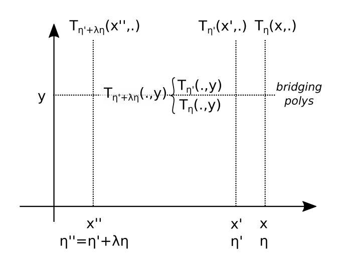
The two replacement steps of inner sumcheck aggregation.
Cross-circuit generalization
The case of several circuits is an immediate generalization of the single circuit case. The accumulator for a collection $\Gamma=\{\Gamma_1,…,\Gamma_M\}$ of circuits keeps track of the cross-circuit linear combination
\[
T_\Gamma(\alpha,Y) = \sum_{k=1}^M \eta_A[k]\cdot A_k(\alpha,Y) + \eta_B[k]\cdot B_k(\alpha,Y) + \eta_C[k]\cdot C_k(\alpha,Y)
\]
through the random coefficients $\eta_A[k],\eta_B[k],\eta_C[k]$ for each of the circuits $\Gamma_k$ separately. (Here, $A_k$, $B_k$, $C_k$ are the R1CS matrices of $\Gamma_k$). As mentioned above, cross-circuit aggregation is useful for schemes with a larger collection of recursive nodes. For example, the block proof of a Latus sidechain is a dynamically arranged tree of Merge-2, Merge-1 and a variety of different base proofs. See our paper Darlin for further details.
Zero-knowledge
A Darlin node is run in zero-knowledge mode whenever it needs to secure private witness data. There are many applications in which zero-knowledge is favourable, such as shielded transactions, zero-knowledge audits or any other type of correctness proof for private state transitions. You may want to read our Zendoo paper if you are interested in where the Zendoo ecosystem applies zero-knowledge.
What else?
The Darlin proof system comes with a few other tweaks. We introduce an alternative way to handle the univariate sumcheck argument, a “cohomological” argument influenced by Plonk. This argument does not rely on individual degree bounds (and their proofs) and allows a more lightweight information-theoretic protocol notion. We also use a slightly different arithmetization for the R1CS matrices. (During the zk-proof workshop we learned that we are not the only ones doing the latter. Lunar uses the same arithmetization — we would like to thank Anaïs Querol for the interesting discussion!)
We believe that Darlin might be useful for other projects which target recursive proofs but still want to stay with R1CS and small proof sizes. And we are curious how Darlin (once our implementation is ready) performs against Plonk based recursive schemes such as Halo 2 or Mina’s Pickles.